NeuralCF

本文主要参考了NeuralCf的论文，及王喆的《深度学习与推荐系统》一书，文中的图片也都来自于此。
NeuralCF论文中文翻译
在前边我们学习了矩阵分解，我们从深度学习视角看待矩阵分解，其中矩阵分解中的用户隐向量和物品隐向量完全可以看作是一种Embedding方法，最终的输出就是用户隐向量和物品隐向量进行内积操作得到最终的评分预测。如果我们用神经网络来描述这个过程的话就是如下图所示：

是不是觉得模型的结构过于简单了呢，两个隐向量之间仅仅通过一个内积就输出了，所以也就会导致矩阵分解模型常常处于欠拟合的状态，无法对优化目标进行有效的拟合。
在NeuralCF的论文中作者也举了一个例子来说明通过内积来预测评分的不可靠性。

上图说明了内积如何限制了MF的表达能力。
为了更好的解释实例，我们明确两种设置：

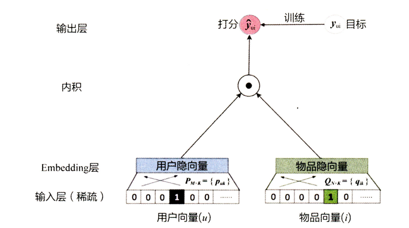
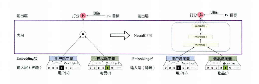
• MF将用户和物品映射到相同的潜在空间中，因此可以用内积衡量两个用户之间的相似性，也可以等效为他们潜在向量之间的夹角的余弦。
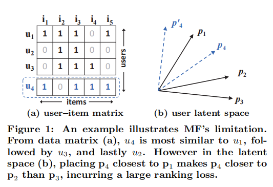
• 使用Jaccard系数作为相似性系数
  

首先，我们关注图(a)的前三行用户，很容易得到$s_{23}(0.66)>s_{12}(0.5)>s_{13}(0.4)$,因此潜在空间中$p_{1},p_{2},p_{3}$的几何关系可以绘制为图(b)所示。现在我们加入一个新用户$u_{4}$，其输入如图(a)虚线所示，我们可以得到 $s_{41}(0.6) > s_{43}(0.4) > s_{42}(0.2)$，这意味着 $u_{4}$ 与 $u_{1}$ 最相似，其次是 $u_{3}$，最后是 $u_{2}$。但是，如果 MF 模型将 p4 放置在最接近 p1 的位置（这两个选项在图 b 中用虚线显示），它将导致 p4 比 p3 更接近 p2，而这会导致很大的排名损失。
于是乎作者认为解决该问题的一个方法是使用大量的潜在因素k(即增大隐向量的个数),但是他可能会对模型的泛化产生不利的影响（例如过拟合）。所以作者通过从数据中使用dnn学习交互函数来解决这个局限性。所以我们的矩阵分解就就变成了下图所示的：

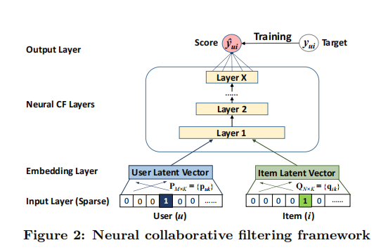
NCF模型

通用框架

为了允许协调过滤进行完整的神经处理，我们采用多层对用户-物品交互进行$y_{ui}$建模,如图所示，其中一层的输出作为下一层的输入，底层输入层有两个特征向量$v_{u}^{U}$和$v_{i}^{I}$分别描述用户u和物品i的特征。在论文中，只使用一个用户的身份和一个项目作为输入特征，将其转换为一个具有one-hot编码的二值化稀疏向量。
在输入层之上的为Embedding层，他是一个全连接层，将稀疏表示投影到稠密向量上。得到的用户(项目)Embedding可以看作是用户(项目)在隐因子模型上下文中的隐向量。然后将用户Embedding和项目Embedding分别注入多层神经网络结构，我们称之为神经协同过滤层，将隐向量映射到预测分数。可以自定义NeuralCF中的每一层，以发现用户-物品交互的某些潜在结构。最后一个隐含层X的维数决定了模型的能力。最后的输出层是预测的分数 $y_{ui}$ ,而训练是通过最小化 ${\hat{y}}_{ui}$ 和 $y_{ui}$ 之间的pointwise loss来完成的。
所以NCF模型可用公式表示为：

$${\hat{y}}_{ui}=f(P^{T}v_{u}^{U},Q^{T}v_{i}^{I}| P,Q,\Theta _{f})$$

这里的$P \in R^{M*K},Q \in R^{N*K}$分别表示用户和物品的隐含因子矩阵。$\Theta_{f}$表示了交互函数f的模型参数。函数f可以定义为多层神经网络，可被表述为：

$$f(P^{T}v_{u}^{U},Q^{T}v_{i}^{I})=\phi_{out}(\phi_{X}(...\phi_{2}(\phi_{1}(P^{T}v_{u}^{U},Q^{T}v_{i}^{I}))...))$$

$\phi_{out},\phi_{x}$分别表示输出层和第x层神经协调过滤的映射函数(CF)层，总共有X个神经CF层。

MCF的学习

为了学习模型参数，现有的pointwise方法大多使用了平方损失的回归：

$$L_{sqr}=\sum_{(u,i)\in y ∪y-}w_{ui}(y_{ui}-{\hat{y_{ui}}})^{2}$$

y表示了在Y中观察到的相互作用的集合，y-表示负向实例的集合。$w_{ui}$是表示训练实例(u, i)权值的超参数。虽然平方损失可以通过假设观测结果是由高斯分布产生来解释，但我们指出它可能与隐式数据不符。这是因为对于隐式数据，目标值 $y_{ui}$是一个二值化的1或0，表示u是否与i交互。

考虑到隐式反馈的一类性质，我们可以将 $y_{ui}$ 的值看作一个标签—1表示物品i与用户u相关，否则为0。预测得分 ${\hat{y}}_{ui}$ 表示了用户u和物品i之间相关-的可能性。赋予NCF这种概率解释,我们需要限制输出${\hat{y}}_{ui}$在[0,1]之间,它可以很容易地通过使用概率函数(例如,Logistic或Probit函数)作为输出层 $\phi_{out}$激活函数。在上述介绍的环境下，定义概率函数如下所示：

$$p(y,y-|P,Q,\Theta_{f})=\prod_{(u,i)\in y}{\hat{y}}_{ui}\prod_{(u,i)\in y-}(1-{\hat{y}}_{ui})$$

取概率的负对数，我们得到：

$$L=-\sum_{(u,i)\in y}log{\hat{y}}_{ui}-\sum_{(u,i)\in y-}log(1-{\hat{y}}_{ui}) =-\sum_{(u,i)\in y \bigcup y-}(y_{ui}log{\hat{y}}_{ui}+(1-y_{ui})log(1-{\hat{y}}_{ui}))$$

这是NCF方法最小化的目标函数，其优化可以通过使用随机梯度下降(SGD)来实现。

这里的代价函数和我们熟悉的二分类交叉熵损失函数是一样的，通过对NCF的概率处理，我们将隐式反馈推荐作为一个二元分类问题。

广义矩阵分解(GMF)

其模型结果如图左边部分所示。由于对输入层的用户(项目)ID进行one-hot编码，得到的Embedding向量可视为用户(项目)的隐向量。设用户的隐向量 $p_{u}$ 为$P^{T}v_{u}^{U}$ ，物品隐向量 $q_{i}$ 为 $Q^{T}v_{v}^{I}$ 。我们定义CF第一层的映射函数为

$$\phi_{1}(p_{u},q_{i})=p_{u}\bigodot q_{i}$$

$\bigodot$表示向量的对应元素相乘，然后我们将向量投影到输出层：

$${\hat{y}}_{ui}=a_{out}(h^{T}(p_{u}\bigodot q_{i}))$$

$a_{out}$ 和h分别表示输出层的激活函数和权值。与普通的MF不同的是， 这里的隐向量进行对应元素相乘之后会有个权重， 也就是各个隐向量维度的重要性不一定相同了。 如果h是一个全1向量并且$a_{out}$是一个恒等函数的话， 那模型实际上就是MF了。在论文中，$a_{out}$被定义为sigmoid函数。

多层感知机(MLP)

由于NCF采用两种路径来对用户和项目进行建模，所以将这两种路径的特征串联起来是很直观的。然而，简单的向量连接并不能解释用户和物品的潜在特征之间的任何交互，这对于协同过滤进行建模效果是不够的。为了解决这个问题，我们建议在连接的向量上添加隐藏层，使用一个标准的MLP来学习用户和物品潜在特征之间的交互。从这个意义上说，我们可以赋予模型很大程度的灵活性和非线性来学习 $p_{u}$和 $q_{i}$ 之间的交互。NCF框架下的MLP模型定义为：

$W_{x},b_{x},a_{x}$分别表示第x层感知器的权值矩阵，偏置向量和激活函数。对于MLP层的激活函数，可以自由选择sigmoid、tanh和ReLU等函数。

GML和MLP融合

GMF采用线性核函数对潜在特征交互进行建模，MLP采用非线性核函数从数据中学习交互函数。接下来的问题是:我们如何在NCF框架下融合GMF和MLP，使得它们可以相互增强，从而更好地对复杂的用户-物品矩阵迭代交互进行建模。
其网络结果在上面的图片中已经给出了，其模型用公式可表示为：

$p_{u}^{G}$ 和 $p_{u}^{M}$ 分别表示GMF部分和MLP部分的用户Embedding，类似的， $q_{i}^{G}$ 和 $q_{i}^{M}$分别表示GMF和MLP的物品Embedding。
我们注意到GML和MLP的Embedding是单独学习的不是独享的,而是单独学习的。作者给出的原因是：共享GMF和MLP的Embedding可能会限制融合模型的性能。例如，它意味着GMF和MLP必须使用相同大小的Embedding;对于两种模型的最优嵌入尺寸变化较大的数据集，该方案可能无法获得最优的集成。为了给融合模型提供更大的灵活性，我们允许GMF和MLP学习独立的Embedding。

预训练

由于NeuMF目标函数的非凸性，基于梯度的优化方法只能找到局部最优解。初始化对深度学习模型的收敛性和性能起着重要的作用。由于NeuMF是一个集成GMF和MLP的模型，我们建议使用GMF和MLP的预训练模型初始化NeuMF。
我们首先用随机初始化训练GMF和MLP，直到收敛。然后，我们使用它们的模型参数作为NeuMF参数的相应部分的初始化。唯一的调整是在输出层，我们将两个模型的权值连接在一起

$$h \gets\begin{bmatrix} \alpha h^{GMF} \\ (1-\alpha)h^{MLP} \end{bmatrix}$$

其中，$h^ {GMF}$和$h^ {MLP}$分别表示预训练的GMF和MLP模型的h向量；α是决定两个预训练模型之间权衡的超参数。
对于GMF和MLP的从无到有的训练，采用了Adam,它通过对频繁的参数执行较小的更新和对不频繁的参数执行较大的更新来适应每个参数的学习率。与普通的SGD相比，Adam方法在两种模型中都能获得更快的收敛速度，并且减轻了调整学习速率的痛苦。

代码

数据处理

import scipy.sparse as sp
import numpy  as np

dataset = 'ml-1m'
main_path = './Data/'
train_rating = main_path + '{}.train.rating'.format(dataset)
test_rating = main_path + '{}.test.rating'.format(dataset)
test_negative = main_path + '{}.test.negative'.format(dataset)

# filename为test.rating的数据   类似于测试集的制作
def load_rating_file_as_list(filename):
    ratingList = []
    with open(filename, "r") as f:
        line = f.readline()
        while line is not None and line != "":
            arr = line.split("\t")
            user, item = int(arr[0]), int(arr[1])
            ratingList.append([user, item])     # 用户名 电影名
            line = f.readline()
    return ratingList

testRatings=load_rating_file_as_list(test_rating)

print(len(testRatings))#共6040行

6040

print(testRatings[0])

[0, 25]

# test.negative
def load_negative_file(filename):
    negativeList = []
    with open(filename, "r") as f:
        line = f.readline()
        while line is not None and line != "":
            arr = line.split("\t")
            negatives = []
            for x in arr[1:]:
                negatives.append(int(x))
            negativeList.append(negatives)
            line = f.readline()
    return negativeList

# test.negative
def load_testdata(filename):
    test_data = []
    with open(filename, "r") as f:
        line = f.readline()
        while line is not None and line != "":
            arr = line.split("\t")
            u=eval(arr[0])[0]
            test_data.append([u, eval(arr[0])[1]])
            for x in arr[1:]:
               test_data.append([u,int(x)])
            line = f.readline()
    return test_data

test_data=load_testdata(filename=test_negative)
print(len(test_data))
print(test_data[0])
print(len(test_data[0]))

604000
[0, 25]
2

np.save('./ProcessedDate/testdate.npy',np.array(test_data))

testNegatives=load_negative_file(test_negative)

print(len(testNegatives))
print(len(testNegatives[0]))
testNegatives[0]#每行99个，即该用户为打过分的电影

6040
99
[1064,
 174,
 2791,
 3373,
 269,
 2678,
 1902,
 3641,
 1216,
...
 58,
 2551,
 2333,
 2688,
 3703,
 1300,
 1924,
 3118]

def load_rating_file_as_matrix(filename):#将测试集的数据转换为稀疏矩阵
    """
    Read .rating file and Return dok matrix.
    The first line of .rating file is: num_users\t num_items
    """
    # Get number of users and items
    num_users, num_items = 0, 0   # 这俩记录用户编号和物品编号里面的最大值
    with open(filename, "r") as f:
        line = f.readline()
        while line is not None and line != "":
            arr = line.split("\t")
            u, i = int(arr[0]), int(arr[1])
            num_users = max(num_users, u)
            num_items = max(num_items, i)
            line = f.readline()
    # Construct matrix
    mat = sp.dok_matrix((num_users + 1, num_items + 1), dtype=np.float32)  # dok_matrix可以高效地逐渐构造稀疏矩阵。 存储是稀疏存储 toarray()
    with open(filename, "r") as f:
        line = f.readline()
        while line is not None and line != "":
            arr = line.split("\t")
            user, item, rating = int(arr[0]), int(arr[1]), float(arr[2])
            if rating > 0:
                mat[user, item] = 1.0
            line = f.readline()
    return mat   # 0,1矩阵， 如果评过分就是1， 否则是0

trainMatrix=load_rating_file_as_matrix(train_rating)

trainMatrix.shape

(6040, 3706)

trainMatrix[0]

<1x3706 sparse matrix of type '<class 'numpy.float32'>'
	with 52 stored elements in Dictionary Of Keys format>

#上述代码可以换成如下
import pandas as pd
train_data=pd.read_csv(train_rating,sep='\t',header=None, names=['user', 'item'], 
    usecols=[0, 1], dtype={0: np.int32, 1: np.int32})
user_number=train_data['user'].max()+1
item_number=train_data['item'].max()+1
train_data=train_data.values.tolist()
trainMatrix1=sp.dok_matrix((user_number,item_number),dtype=np.float32)
for train in train_data:
    trainMatrix1[train[0],train[1]]=1.0

print(len(train_data))

994169

train_data=pd.read_csv(train_rating,sep='\t',header=None, names=['user', 'item'], 
    usecols=[0, 1], dtype={0: np.int32, 1: np.int32})

index=train_data[(train_data.user==549)&(train_data['item']==1543)].index.tolist()
train_data.loc[index,:]

	user	item
83241	549	1543

train_datalist=train_data.values.tolist()
train_datalist[:20]

[[0, 32],
 [0, 34],
 [0, 4],
 [0, 35],
 [0, 30],
 [0, 29],
 [0, 33],
 [0, 40],
 [0, 10],
 [0, 16],
 [0, 23],
 [0, 28],
 [0, 12],
 [0, 8],
 [0, 5],
 [0, 20],
 [0, 46],
 [0, 15],
 [0, 50],
 [0, 49]]

np.save('./ProcessedDate/train_datalist.npy',np.array(train_datalist))

trainMatrix1.shape

(6040, 3706)

trainMatrix1[0]

<1x3706 sparse matrix of type '<class 'numpy.float32'>'
	with 52 stored elements in Dictionary Of Keys format>

# 下面把上面的三个矩阵保存  注意得保存成numpy的形式
np.save('./ProcessedDate/trainMatrix.npy',trainMatrix1)
np.save('./ProcessedDate/testRatings.npy',np.array(testRatings))
np.save('./ProcessedDate/testNegatives.npy',np.array(testNegatives))

####导包

import datetime
import numpy as np
import pandas as pd
from collections import Counter
import heapq

import torch
from torch.utils.data import DataLoader, Dataset, TensorDataset

import torch.nn as nn
import torch.nn.functional as F
import torch.optim as optim

#from torchkeras import summary,KerasModel

import warnings
warnings.filterwarnings('ignore')

import torch.utils.data as data

device = torch.device("cuda:0" if torch.cuda.is_available() else "cpu")
```python
# 一些超参数设置
# 一些超参数设置
topK = 10
num_factors = 8
num_negatives = 4
batch_size = 64
lr = 0.001
layers=[num_factors*2,64,32,16,8]

从文件中导入数据进行处理

导入数据

train=np.load(‘./ProcessedDate/trainMatrix.npy’,allow_pickle=True).tolist()
train_datalist=np.load(‘./ProcessedDate/train_datalist.npy’).tolist()
testRatings = np.load(‘./ProcessedDate/testRatings.npy’).tolist()
testNegatives = np.load(‘./ProcessedDate/testNegatives.npy’).tolist()
model_path=‘./models/’

```python
type(train)

scipy.sparse._dok.dok_matrix

train.count_nonzero()

994169

train_data=train_datalist

type(train_data)
print(len(train_data))
train_data[0]

994169





[0, 32]

num_users, num_items = train.shape
num_users

6040

将数据送入dataloader

# 根据继承pytorch的Dataset类定义数据类
class CFData(data.Dataset):
    def __init__(self, features,
                 num_item, train_mat=None, num_ng=0, is_training=None):
        """features=train_data,num_item=item_num,train_mat，稀疏矩阵，num_ng,训练阶段默认为4，即采样4-1个负样本对应一个评分过的
        数据。
        """
        super(CFData, self).__init__()
        """ Note that the labels are only useful when training, we thus 
            add them in the ng_sample() function.
        """
        self.features = features
        self.num_item = num_item
        self.train_mat = train_mat
        self.num_ng = num_ng
        self.is_training = is_training

    def ng_sample(self):
        assert self.is_training, 'no need to sampling when testing'

        self.features_fill = []
        for (u,i) in self.train_mat.keys():
            self.features_fill.append([u,i,1])


            for t in range(self.num_ng):
                j=np.random.randint(self.num_item)
                while (u,j) in self.train_mat:
                    j=np.random.randint(self.num_item)
                self.features_fill.append([u,j,0])

        # for x in self.features:
        #     u, i = x[0], x[1]
        #     for t in range(self.num_ng):
        #         j = np.random.randint(self.num_item)
        #         while (u, j) in self.train_mat:
        #             j = np.random.randint(self.num_item)
        #         self.features_fill.append([u, i, j])

    def __len__(self):
        return self.num_ng * len(self.features) if \
            self.is_training else len(self.features)

    def __getitem__(self, idx):
        features = self.features_fill if \
            self.is_training else self.features
        

        user = features[idx][0]
        item_i = features[idx][1]
        if self.is_training:
            labels=features[idx][2]
        else:
            if idx%100==0:
                labels=1
            else:
                labels=0
    
        return user, item_i, labels

train_dataset = CFData(
        train_data, num_item=num_items, train_mat=train, num_ng=4, is_training=True)
train_loader=DataLoader(train_dataset,batch_size=batch_size,shuffle=True)

#测试一下
train_loader.dataset.ng_sample()
for (x,y,z) in (train_loader):
    print(x,y,z)
    break
print(x.shape)
print(y.shape)
print(z.shape)

tensor([2806, 4053, 1088, 2453, 4214, 4276,  300, 4193, 3642, 3311, 2461, 4470,
        3328, 2811,  255,  797, 3568,  548, 3128, 4052,  769, 3161, 2430,  838,
        2736, 3355,  328, 2241, 3257, 2615, 3475, 2888, 3223, 3155, 4203, 1946,
        2241, 2800, 3310, 1424, 4678,  562, 4770, 3689, 3104, 1997,  711, 1316,
        2628, 2963, 4747, 2244, 3765, 1469, 1028, 3390,  939, 4052, 1054, 1223,
        3280, 1477,  186,  586]) tensor([ 334, 2581, 3629, 3139, 3470, 1796, 1147, 1446, 2966, 3677, 1369,  968,
        3537,  417,  628,  455, 2118, 1850, 2436, 1830, 2225, 2774, 1351, 1606,
        1596, 1859, 2455, 2854, 1495,  337, 3214,  675, 1284,  979,  449,  211,
         616, 1061, 3352, 3418,  933, 2505, 3393,  496,  381,  520, 3445,  155,
        1393, 2275, 2432, 2389, 3186, 2265, 2652, 2692, 2590,  231, 2934,   97,
        1008, 3598, 2490, 2178]) tensor([0, 0, 0, 0, 0, 0, 0, 0, 0, 0, 0, 0, 0, 0, 0, 0, 0, 1, 0, 0, 0, 0, 0, 0,
        1, 0, 0, 0, 0, 1, 0, 0, 1, 1, 0, 1, 1, 0, 0, 0, 1, 0, 0, 0, 1, 1, 0, 1,
        0, 0, 0, 0, 0, 1, 0, 0, 0, 0, 0, 1, 0, 0, 0, 0])
torch.Size([64])
torch.Size([64])
torch.Size([64])

定义模型

MLP

##定义模型
class MLP(nn.Module):
    def __init__(self,num_users,num_items,factor_num=32,layers=[20,64,32,16],regs=[0,0]):
        super(MLP,self).__init__()
        
        self.MF_Embedding_User=nn.Embedding(num_embeddings=num_users,embedding_dim=factor_num)
        self.MF_Embedding_Item=nn.Embedding(num_embeddings=num_items,embedding_dim=factor_num)

        #全连接层
        self.dnn_network = nn.ModuleList([nn.Linear(layer[0], layer[1]) for layer in list(zip(layers[:-1], layers[1:]))])
        self.linear=nn.Linear(layers[-1],1)
        self.sigmoid=nn.Sigmoid()

    def forward(self,inputs):
        # 这个inputs是一个批次的数据， 所以后面的操作切记写成inputs[0], [1]这种， 这是针对某个样本了， 我们都是对列进行的操作
        # 先把输入转成long类型
        inputs=inputs.long()


        #前向传播
        MF_Embedding_User=self.MF_Embedding_User(inputs[:,0])
        MF_Embedding_Item=self.MF_Embedding_Item(inputs[:,1])

        #两个隐向量叠加
        x=torch.cat([MF_Embedding_User,MF_Embedding_Item],dim=-1)

        #全连接层
        for linear in self.dnn_network:
            x=linear(x)
            x=F.relu(x)
        
        x=self.linear(x)

        predictions=self.sigmoid(x)
        predictions = predictions.squeeze(-1)

        predictions=predictions.float()
        return predictions

#定义模型
model=MLP(num_users=num_users,num_items=num_items,factor_num=num_factors,layers=layers)
model.to(device=device)

MLP(
  (MF_Embedding_User): Embedding(6040, 8)
  (MF_Embedding_Item): Embedding(3706, 8)
  (dnn_network): ModuleList(
    (0): Linear(in_features=16, out_features=64, bias=True)
    (1): Linear(in_features=64, out_features=32, bias=True)
    (2): Linear(in_features=32, out_features=16, bias=True)
    (3): Linear(in_features=16, out_features=8, bias=True)
  )
  (linear): Linear(in_features=8, out_features=1, bias=True)
  (sigmoid): Sigmoid()
)

x=x.reshape((-1,1))
y=y.reshape((-1,1))
a=torch.cat((x,y),dim=-1)

#测试一下模型
print(model(a))
model(a)[0]

tensor([0.4523, 0.4545, 0.4527, 0.4530, 0.4540, 0.4600, 0.4537, 0.4567, 0.4529,
        0.4557, 0.4526, 0.4551, 0.4532, 0.4532, 0.4549, 0.4571, 0.4519, 0.4547,
        0.4545, 0.4538, 0.4538, 0.4548, 0.4574, 0.4529, 0.4519, 0.4539, 0.4534,
        0.4551, 0.4523, 0.4524, 0.4547, 0.4527, 0.4564, 0.4514, 0.4603, 0.4538,
        0.4542, 0.4539, 0.4532, 0.4548, 0.4549, 0.4527, 0.4529, 0.4532, 0.4569,
        0.4534, 0.4536, 0.4524, 0.4545, 0.4561, 0.4527, 0.4539, 0.4546, 0.4542,
        0.4562, 0.4547, 0.4533, 0.4521, 0.4555, 0.4517, 0.4553, 0.4518, 0.4521,
        0.4526], grad_fn=<SqueezeBackward1>)





tensor(0.4523, grad_fn=<SelectBackward0>)

GMF

class GMF(nn.Module):
    def __init__(self,num_uers,num_items,factor_numbers=32):
        super(GMF,self).__init__()
        self.MF_Embedding_User=nn.Embedding(num_uers,embedding_dim=factor_numbers)
        self.MF_Embedding_Item=nn.Embedding(num_items,factor_numbers)
        self.linear=nn.Linear(factor_numbers,1)
        self.sigmoid=nn.Sigmoid()
    
    def forward(self,inputs):
        
        #Embedding层必须是long类型数据，否则会报错
        inputs=inputs.long()

        MF_Embedding_User=self.MF_Embedding_User(inputs[:,0])
        MF_Embedding_Item=self.MF_Embedding_Item(inputs[:,1])
        predict_vec=torch.mul(MF_Embedding_User,MF_Embedding_Item)

        linear=self.linear(predict_vec)
        output=self.sigmoid(linear)
        
        #将最终结果从二维转换为一维
        output=output.squeeze(-1)
        return output

model=GMF(num_users,num_items,num_factors)
model.to(device)

GMF(
  (MF_Embedding_User): Embedding(6040, 8)
  (MF_Embedding_Item): Embedding(3706, 8)
  (linear): Linear(in_features=8, out_features=1, bias=True)
  (sigmoid): Sigmoid()
)

x=x.reshape((-1,1))
y=y.reshape((-1,1))
a=torch.cat((x,y),dim=-1)
print(model(a))

tensor([0.3108, 0.3083, 0.6403,  ..., 0.8549, 0.8039, 0.3121],
       grad_fn=<SqueezeBackward1>)

NMF

class NeuralMF(nn.Module):
    def __init__(self,num_users,num_items,mf_dim,layers):
        super(NeuralMF,self).__init__()

        self.MF_Embedding_User=nn.Embedding(num_users,mf_dim)
        self.MF_Embedding_Item=nn.Embedding(num_items,mf_dim)

        self.MLP_Embedding_User=nn.Embedding(num_users,layers[0] //2)
        self.MLP_Embedding_Item=nn.Embedding(num_items,layers[0]//2)


        self.dnn_network=nn.ModuleList([nn.Linear(layer[0], layer[1]) for layer in list(zip(layers[:-1], layers[1:]))])
        self.linear=nn.Linear(layers[-1],mf_dim)

        #合并之后
        self.linear2=nn.Linear(2*mf_dim,1)
        self.sigmoid=nn.Sigmoid()

    def forward(self,inputs):
        
        inputs=inputs.long()

        MF_Embedding_User=self.MF_Embedding_User(inputs[:,0])
        MF_Embedding_Item=self.MF_Embedding_Item(inputs[:,1])

        mf_vec=torch.mul(MF_Embedding_User,MF_Embedding_Item)

        MLP_Embedding_User=self.MLP_Embedding_User(inputs[:,0])
        MLP_Embedding_Item=self.MLP_Embedding_Item(inputs[:,1])

        x=torch.cat([MLP_Embedding_User,MLP_Embedding_Item],dim=-1)

        #print(x.shape)
        for linear in self.dnn_network:
            x=linear(x)
            x=F.relu(x)
        
        mlp_vec=self.linear(x)

        #合并两个

        vector=torch.cat([mf_vec,mlp_vec],dim=-1)
        linear=self.linear2(vector)
        output=self.sigmoid(linear)
        
        output=output.squeeze(-1)
        return output

model=NeuralMF(num_users,num_items,num_factors,layers)
model.to(device)

NeuralMF(
  (MF_Embedding_User): Embedding(6040, 8)
  (MF_Embedding_Item): Embedding(3706, 8)
  (MLP_Embedding_User): Embedding(6040, 8)
  (MLP_Embedding_Item): Embedding(3706, 8)
  (dnn_network): ModuleList(
    (0): Linear(in_features=16, out_features=64, bias=True)
    (1): Linear(in_features=64, out_features=32, bias=True)
    (2): Linear(in_features=32, out_features=16, bias=True)
    (3): Linear(in_features=16, out_features=8, bias=True)
  )
  (linear): Linear(in_features=8, out_features=8, bias=True)
  (linear2): Linear(in_features=16, out_features=1, bias=True)
  (sigmoid): Sigmoid()
)

model(a)

tensor([0.5335, 0.6584, 0.6141, 0.5763, 0.4243, 0.5309, 0.5333, 0.4247, 0.5536,
        0.5929, 0.5608, 0.5473, 0.5609, 0.5059, 0.5331, 0.5905, 0.5931, 0.5454,
        0.4831, 0.5259, 0.5547, 0.5405, 0.5677, 0.6399, 0.5988, 0.5861, 0.5574,
        0.5722, 0.5028, 0.7629, 0.5612, 0.6122, 0.4081, 0.6269, 0.5933, 0.6069,
        0.6996, 0.6164, 0.5964, 0.5967, 0.6911, 0.5107, 0.5526, 0.5478, 0.5358,
        0.5651, 0.4293, 0.4630, 0.4618, 0.5442, 0.5680, 0.5080, 0.5040, 0.5064,
        0.5338, 0.5138, 0.5314, 0.4367, 0.7294, 0.4487, 0.5008, 0.6045, 0.5884,
        0.4132], grad_fn=<SqueezeBackward1>)

定义评价指标

# Global variables that are shared across processes
_model = None
_testRatings = None
_testNegatives = None
_K = None

# HitRation
def getHitRatio(ranklist, gtItem):
    for item in ranklist:
        if item == gtItem:
            return 1
    return 0

# NDCG
def getNDCG(ranklist, gtItem):
    for i in range(len(ranklist)):
        item = ranklist[i]
        if item == gtItem:
            return np.log(2) / np.log(i+2)
    return 0

def eval_one_rating(idx):   # 一次评分预测
    rating = _testRatings[idx]
    items = _testNegatives[idx]
    u = rating[0]
    gtItem = rating[1]
    items.append(gtItem)
    
    # Get prediction scores
    map_item_score = {}
    users = np.full(len(items), u, dtype='int32')
    
    test_data = torch.tensor(np.vstack([users, np.array(items)]).T).to(device)
    predictions = _model(test_data)
    for i in range(len(items)):
        item = items[i]
        map_item_score[item] = predictions[i].data.cpu().numpy()
    items.pop()
    
    # Evaluate top rank list
    ranklist = heapq.nlargest(_K, map_item_score, key=lambda k: map_item_score[k])  # heapq是堆排序算法， 取前K个
    hr = getHitRatio(ranklist, gtItem)
    ndcg = getNDCG(ranklist, gtItem)
    return hr, ndcg

def evaluate_model(model, testRatings, testNegatives, K):
    """
    Evaluate the performance (Hit_Ratio, NDCG) of top-K recommendation
    Return: score of each test rating.
    """
    global _model
    global _testRatings
    global _testNegatives
    global _K
    
    _model = model
    _testNegatives = testNegatives
    _testRatings = testRatings
    _K = K
    
    hits, ndcgs = [], []
    for idx in range(len(_testRatings)):
        (hr, ndcg) = eval_one_rating(idx)
        hits.append(hr)
        ndcgs.append(ndcg)
    return hits, ndcgs   

#测试一下
(hits, ndcgs) = evaluate_model(model, testRatings, testNegatives, topK)
hr, ndcg = np.array(hits).mean(), np.array(ndcgs).mean()
print('Init: HR=%.4f, NDCG=%.4f' %(hr, ndcg))

Init: HR=0.1017, NDCG=0.0466

训练

定义优化器

# 训练参数设置
loss_func = nn.BCELoss()#二分类交叉熵损失函数
optimizer = torch.optim.Adam(params=model.parameters(), lr=lr)

训练模型

这里以其中一个模型为例，展示训练过程

# 模型训练 
import time
best_hr, best_ndcg, best_iter = hr, ndcg, -1

epochs = 20
log_step_freq = 10000

for epoch in range(epochs):
    
    # 训练阶段
    model.train()
    loss_sum = 0.0
    start_time=time.time()
    train_loader.dataset.ng_sample()
    step=0
    for user,item,labels in train_loader:
        step+=1
        user=user.to(device)
        item=item.to(device)
        labels=labels.to(device)
        
        # 梯度清零
        model.zero_grad()
        # x=x.reshape((-1,1))
        # y=y.reshape((-1,1))
        # a=torch.cat((x,y),dim=-1)
        user=user.reshape((-1,1))
        item=item.reshape((-1,1))
        features=torch.cat((user,item),dim=-1)
        
        # 正向传播
        predictions = model(features)
        
        predictions=predictions.to(torch.float32)
        labels=labels.to(torch.float32)
        
        loss = loss_func(predictions, labels)
        
        # 反向传播求梯度
        loss.backward()
        optimizer.step()
        
        # 打印batch级别日志
        loss_sum += loss.item()
        if step % log_step_freq == 0:
            print(("[step = %d] loss: %.3f") %
                  (step, loss_sum/step))
    
    # 验证阶段
    model.eval()
    (hits, ndcgs) = evaluate_model(model, testRatings, testNegatives, topK)
    hr, ndcg = np.array(hits).mean(), np.array(ndcgs).mean()
    elapsed_time=time.time()-start_time
    print("The time elapse of epoch {:03d}".format(epoch) + " is: " +
         time.strftime("%H: %M: %S", time.gmtime(elapsed_time)))
    if hr > best_hr:
        best_hr, best_ndcg, best_iter = hr, ndcg, epoch
        torch.save(model.state_dict(), 'Pre_train/m1-1m_NeuralMF.pkl')  
        
    info = (epoch, loss_sum/step, hr, ndcg)
    print(("\nEPOCH = %d, loss = %.3f, hr = %.3f, ndcg = %.3f") %info)
print('Finished Training...') 

[step = 10000] loss: 0.263
[step = 20000] loss: 0.263
[step = 30000] loss: 0.264
[step = 40000] loss: 0.264
[step = 50000] loss: 0.264
[step = 60000] loss: 0.264
The time elapse of epoch 000 is: 00: 02: 52

EPOCH = 0, loss = 0.264, hr = 0.557, ndcg = 0.315
[step = 10000] loss: 0.261
[step = 20000] loss: 0.262
[step = 30000] loss: 0.262
[step = 40000] loss: 0.263
[step = 50000] loss: 0.263
[step = 60000] loss: 0.263
The time elapse of epoch 001 is: 00: 02: 51

EPOCH = 1, loss = 0.263, hr = 0.552, ndcg = 0.313
[step = 10000] loss: 0.260
[step = 20000] loss: 0.261
[step = 30000] loss: 0.262
[step = 40000] loss: 0.262
[step = 50000] loss: 0.262
[step = 60000] loss: 0.262
The time elapse of epoch 002 is: 00: 02: 52

EPOCH = 2, loss = 0.263, hr = 0.550, ndcg = 0.314
[step = 10000] loss: 0.259
[step = 20000] loss: 0.260
[step = 30000] loss: 0.261
[step = 40000] loss: 0.261
[step = 50000] loss: 0.262
[step = 60000] loss: 0.262
The time elapse of epoch 003 is: 00: 02: 50

EPOCH = 3, loss = 0.262, hr = 0.533, ndcg = 0.303
[step = 10000] loss: 0.259
[step = 20000] loss: 0.259
[step = 30000] loss: 0.260
[step = 40000] loss: 0.260
[step = 50000] loss: 0.261
[step = 60000] loss: 0.261
The time elapse of epoch 004 is: 00: 02: 50

EPOCH = 4, loss = 0.261, hr = 0.528, ndcg = 0.302